Optimizing Closed Loop Performance

This tutorial shows how to retrieve data from the ONIX hardware as quickly as possible for experiments with strict low-latency closed-loop requirements by tuning the workflow for your particular data sources and computer specifications. In most situations, sub-200 microsecond closed-loop response times can be achieved.

Note

Performance will vary based on your computer's capabilities and your results might differ from those presented below. The computer used to create this tutorial has the following specs:

• CPU: Intel i9-12900K
• RAM: 64 GB
• GPU: NVIDIA GTX 1070 8GB
• OS: Windows 11

Data Transmission from ONIX Hardware to Host Computer

ONIX is capable of transferring data directly from production to the host computer. However, if the host is busy when ONIX starts producing data, ONIX will temporarily store this new data in its hardware buffer while it waits for the host to be ready to accept new data.

Key details about this process:

• The size of hardware-to-host data transfers is determined by the ReadSize property of the StartAcquisition operator which is in every Bonsai workflow that uses OpenEphys.Onix1 to acquire data from ONIX.
• Increasing ReadSize allows the host to read larger chunks of data from ONIX per read operation without significantly increasing the duration of the read operation, therefore increasing the maximum rate at which data can be read.
• If the host is busy or cannot perform read operations rapidly enough to keep up with the rate at which ONIX produces data, the ONIX hardware buffer will start to accumulate excessive data.
• Accumulation of excess data in the hardware buffer collapses real-time performance and risks hardware buffer overflow which would prematurely terminate the acquisition session. ReadSize can be increased to avoid this situation.
• As long as this situation is avoided, decreasing ReadSize means that ONIX doesn't need to produce as much data before the host can access it. This, in effect, means software can start operating on data closer to the time that the data was produced, thus achieving lower-latency feedback-loops.

In other words, a small ReadSize can help the host access data sooner to when that data was created. However, each data transfer incurs overhead. If ReadSize is so small that ONIX produces a ReadSize amount of data faster than the average time it takes the host computer to perform a read operation, the hardware buffer will accumulate excessive data. This will destroy real-time performance and eventually cause the hardware buffer to overflow, terminating acquisition. The goal of this tutorial is to tune StartAcquisition's ReadSize so that data flows from production to the software running on the host as quickly as possible by minimizing the amount of time that it sits idly in both the ONIX hardware buffer and the host computer's buffer. This provides software access to the data as close to when the data was produced as possible which helps achieve lower latency closed-loop feedback.

Technical Details

Note

This section explains more in-depth how data is transferred from ONIX to the host computer. Although these details provide additional context about ONIX, they are more technical and are not required for following the rest of the tutorial.

When the host computer reads data from the ONIX hardware, it retrieves a ReadSize-bytes sized chunk of data using the following procedure:

1. A ReadSize-bytes long block of memory is allocated on the host computer's RAM by the host API for the purpose of holding incoming data from ONIX.
2. A pointer to that memory is provided to the RIFFA driver (the PCIe backend/kernel driver for the ONIX system) which moves the allocated memory block into a more privileged state known as kernel mode so that it can initiate a DMA transfer. DMA allows data transfer to be performed by ONIX hardware without additional CPU intervention.
3. The data transfer completes once this block of data has been populated with ReadSize bytes of data from ONIX.
4. The RIFFA driver moves the memory block from kernel mode to user mode so that it can be accessed by software. The API function returns with a pointer to the filled buffer.

During this process, memory is allocated only once by the API, and the transfer is zero-copy. The API-allocated buffer is written autonomously by ONIX hardware using minimal resources from the host computer.

So far, all this occurs on the host-side. Meanwhile, on the ONIX-side:

• If ONIX produces new data before the host is able to consume the data in the API-allocated buffer, this new data is added to the back of ONIX hardware buffer FIFO. The ONIX hardware buffer consists of 2GB of RAM that belongs to the acquisition hardware (it is not RAM in the host computer) dedicated to temporarily storing data that is waiting to be transferred to the host. Data is removed from the front of the hardware buffer and transferred to the host once it's ready to accept more data.
• If the memory is allocated on the host-side and the data transfer is initiated by the host API before any data is produced, ONIX transfers new data directly to the host bypassing the hardware buffer. In this case, ONIX is literally streaming data to the host the moment it is produced. This data becomes available for reading by the host once ONIX transfers the full ReadSize bytes.

Tuning ReadSize to Optimize Closed Loop Performance

ONIX provides a mechanism for tuning the value of ReadSize to optimize closed loop performance that takes into account the idiosyncrasies of your host computer and experimental acquisition setup.

Note

If you are not familiar with the basic usage of the OpenEphys.Onix1 library, then visit the Getting Started guide to set up your Bonsai environment and familiarize yourself with using the library to acquire data from ONIX before proceeding.

Copy the following workflow into the Bonsai workflow editor by hovering over the workflow image and clicking on the clipboard icon that appears. Open Bonsai and paste this workflow by clicking the Bonsai workflow editor pane and pressing Ctrl+V.

Hardware Configuration

The top-row configuration chain includes a ConfigureLoadTester operator. This configures ONIX's Load Tester Device, which produces and consumes data at user-specified rates for testing and tuning the latency between data production and real-time feedback. This device is not an emulator. It is a real hardware device that produces and consumes data using the selected driver and physical link (e.g. PCIe bus) and thus provides accurate measurements of feedback performance for a given host computer.

We need to configure the load tester to produce and consume the same amount of data as our real experimental hardware would. For example, lets say that during our closed loop experiment, feedback signals will be generated as a function of data acquired from two Neuropixels 2.0 probes, each of which generates a 384 channel sample at 30 kHz. The overall bandwidth is

\[ \begin{equation} 2\,probes*\frac{384\,chan.}{probe}*\frac{30\,ksamp.}{sec\,chan.}*\frac{2\,bytes}{samp.} \approx 47\,MB/s \label{eq:2xnpx2bw} \end{equation} \]

To understand how we came up with this calculation, visit the Data Elements page.

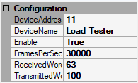
We'll setup ConfigureLoadTester to produce data at the same frequency and bandwidth as two Neuropixels 2.0 probes with the following settings:

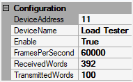
• DeviceAddress is set to 11 because that's how this device is indexed in the ONIX system.
• DeviceName is set to "Load Tester"
• Enable is set to True to enable the LoadTester device.
• FramesPerSecond is then set to 60,000 Hz. The rate at which frames are produced by two probes, since each is acquired independently.
• ReceivedWords is set to 392 bytes, the size of a single NeuropixelsV2eDataFrame including its clock members.
• TransmittedWords is set to 100 bytes. This simulates the amount of data required to e.g. send a stimulus waveform.

Note

The DeviceAddress must be manually configured because ConfigureLoadTester is used for diagnostics and testing and therefore is not made available through ConfigureBreakoutBoard like the rest of the local devices (analog IO, digital IO, etc.). The device address can be found using oni-repl.

Next we configure StartAcquisition's ReadSize and WriteSize properties.

WriteSize is set to 16384 bytes. This defines a readily-available pool of memory for the creation of output data frames. Data is written to hardware as soon as an output frame has been created, so the effect on real-time performance is typically not as large as that of the ReadSize property.

To start, ReadSize is also set to 16384. Later in this tutorial, we'll examine the effect of this value on real-time performance.

Real-time Loop

The bottom half of the workflow is used to stream data back to the load testing device from hardware so that it can perform a measurement of round trip latency. The LoadTesterData operator acquires a sequence of LoadTesterDataFrames from the hardware each of which is split into its HubClock member and HubClockDelta member.

The HubClock member indicates the acquisition clock count when the LoadTesterDataFrame was produced. The EveryNth operator is a Condition operator which only allows through every Nth element in the observable sequence. This is used to simulate an algorithm, such as spike detection, that only triggers closed loop feedback in response to input data meeting some condition. The value of N can be changed to simulate different feedback frequencies. You can inspect its logic by double-clicking the node when the workflow is not running. In this case, N is set to 100, so every 100th sample is delivered to LoadTesterLoopback.

LoadTesterLoopback is a sink which writes HubClock values it receives back to the load tester device. When the load tester device receives a HubClock from the host computer, it's subtracted from the current acquisition clock count. That difference is sent back to the host computer as the HubClockDelta property of subsequent LoadTesterDataFrames. In other words, HubClockDelta indicates the amount of time that has passed since the creation of a frame in hardware and the receipt of a feedback signal in hardware based on that frame: it is a complete measurement of closed loop latency. This value is converted to milliseconds and then Histogram1D is used to help visualize the distribution of closed-loop latencies.

Finally, at the bottom of the workflow, a MemoryMonitorData operator is used to examine the state of the hardware buffer. To learn about the MemoryMonitorData branch, visit the Breakout Board Memory Monitor page.

Relevant Visualizers

The desired output of this workflow are the visualizers for the Histogram1D and PercentUsed nodes. Below is an example of each which we will explore more in the next section:

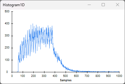
The Histogram1D visualizer shows the distribution of closed-loop feedback latencies. The x-axis is in units of μs, and the y-axis represents the number of samples in a particular bin. The histogram is configured to have 1000 bins between 0 and 1000 μs. For low-latency closed-loop experiments, the goal is to concentrate the distribution of closed-loop feedback latencies towards 0 μs as much as possible.

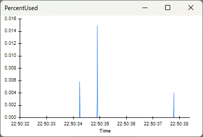
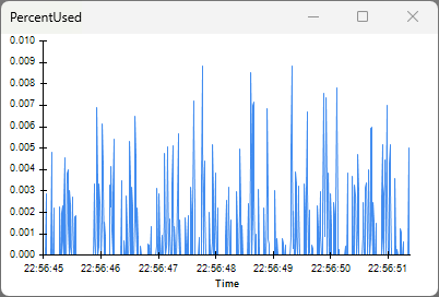
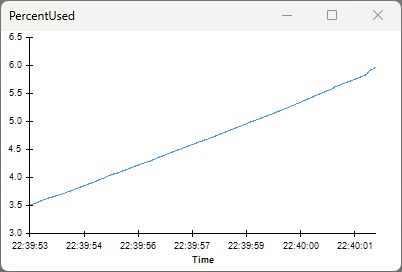
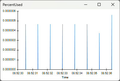
The PercentUsed visualizer shows a time-series of the amount of the hardware buffer that is occupied by data as a percentage of the hardware buffer's total capacity. The x-axis is timestamps, and the y-axis is percentage. To ensure data is available as soon as possible from when it was produced and avoid potential buffer overflow, the goal is to maintain the percentage at or near zero.

Real-time Latency for Different ReadSize Values

ReadSize = 16384 bytes

With ReadSize set to 16384 bytes, start the workflow and open the visualizers for the PercentUsed and Histogram1D nodes:

The Histogram1D visualizer shows that the average latency is about 300 μs, with most latencies ranging from ~60 μs to ~400 μs. This roughly matches our expectations. Since data is produced at about 47MB/s, it takes about 340 μs to produce 16384 bytes of data. This means that the data contained in a single ReadSize block was generated in the span of approximately 340 μs. Because we are using every 100th sample to generate feedback, the sample that is actually used to trigger LoadTesterLoopback could be any from that 340 μs span resulting in a range of latencies. The long tail in the distribution corresponds to instances when the hardware buffer was used or the CPU was busy with other tasks.

The PercentUsed visualizer shows that the percent of the hardware buffer being used remains close to zero. This indicates minimal usage of the hardware buffer, and that the host is safely reading data faster than the ONIX produces that data. For experiments without hard real-time constraints, this latency is perfectly acceptable.

For experiments with harder real-time constraints, let's see how much lower we can get the closed-loop latency.

ReadSize = 2048 bytes

Set ReadSize to 2048 bytes, restart the workflow (ReadSize is a Configuration property so it only updates when a workflow starts), and open the same visualizers:

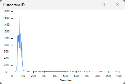
The Histogram1D visualizer shows closed-loop latencies now average about 80 μs with lower variability.

The PercentUsed visualizer shows the hardware buffer is still stable at around zero. This means that, even with the increased overhead associated with a smaller ReadSize, the host is reading data rapidly enough to prevent excessive accumulation in the hardware buffer. Let's see if we can decrease latency even further.

ReadSize = 1024 bytes

Set ReadSize to 1024 bytes, restart the workflow, and open the same visualizers.

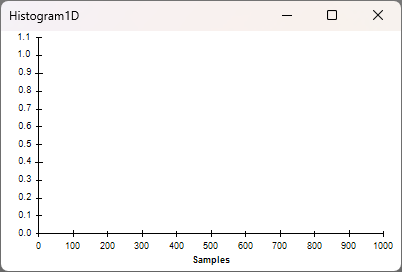
The Histogram1D visualizer appears to be empty. This is because the latency immediately exceeds the x-axis upper limit of 1 ms. You can see this by inspecting the visualizer for the node prior to Histogram1D. Because of the very small buffer size (which is on the order of a single Neuropixels 2.0 sample), the computer cannot perform read operations at a rate required to keep up with data production. This causes excessive accumulation of data in the hardware buffer. In this case, when new data is produced, it gets added to the end of the hardware buffer queue, requiring several read operations before this new data can be read. As more data accumulates in the buffer, the duration of time from when that data was produced and when that data can finally be read increases. In other words, latencies increase dramatically, and closed loop performance collapses.

The PercentUsed visualizer shows that the percentage of the hardware buffer that is occupied is steadily increasing. The acquisition session will eventually terminate in an error when the MemoryMonitor PercentUsed reaches 100% and the hardware buffer overflows.

Summary

The results of our experimentation are as follows:

ReadSize	Latency	Buffer Usage	Notes
16384 bytes	~300 μs	Stable at 0%	Perfectly adequate if there are no strict low latency requirements, lowest risk of buffer overflow
2048 bytes	~80 μs	Stable near 0%	Balances latency requirements with low risk of buffer overflow
1024 bytes	Rises steadily	Unstable	Certain buffer overflow and terrible closed loop performance

These results may differ for your experimental system. For example, your system might have different bandwidth requirements (if you are using different devices, data is produced at a different rate) or use a computer with different performance capabilities (which changes how quickly read operations can occur). For example, here is a similar table made by configuring the Load Tester device to produce data at a rate similar to a single 64-channel Intan chip (such as what is on the Headstage 64), ~4.3 MB/s:

ReadSize	Latency	Buffer Usage	Notes
1024 bytes	~200 μs	Stable at 0%	Perfectly adequate if that are no strict low latency requirements
512 bytes	~110 μs	Stable at 0%	Lower latency, no risk of buffer overflow
256 bytes	~80 μs	Stable at 0%	Lowest achievable latency with this setup, still no risk of buffer overflow
128 bytes	-	-	Results in error -- 128 bytes is too small for the current hardware configuration

Regarding the last row of the above table, the lowest ReadSize possible is determined by the size of the largest data frame produced by enabled devices (plus some overhead). Even with the lowest possible ReadSize value, 256 bytes, there is very little risk of overflowing the buffer. The PercentUsed visualizer shows that the hardware buffer does not accumulate data:

Tip

• The only constraint on ReadSize is the lower limit as demonstrated in the example of tuning for ReadSize for a single 64-channel Intan chip. We only tested ReadSize values that are a power of 2, but ReadSize can be fine-tuned further to achieve even tighter latencies if necessary.
• As of OpenEphys.Onix1 0.7.0: As long as you stay above the minimum mentioned in the previous bullet point, ReadSize can be set to any value by the user. The OpenEphys.Onix1 Bonsai package will round this ReadSize to the nearest multiple of four and uses that value instead. For example, if you try to set ReadSize to 887, the software will use the value 888 instead.
• If you are using a data I/O operator that has capacity to produce data at various rates (like DigitalInput), test your chosen ReadSize by configuring the load tester to produce data at the lower and upper limits that you expect data to be produced during your experiment. This will help ensure excess data doesn't accumulate in the hardware buffer and desired closed-loop latencies are maintained throughout the range of data throughput of these devices.
• Running other processes that demand the CPU's attention might cause spurious spikes in data accumulation in the hardware buffer. Either reduce the amount other processes or test that they don't interfere with your experiment.

These two tables together demonstrate why it is impossible to recommend a single correct value for ReadSize that is adequate for all experiments. The diversity of experiments (in particular, the wide range at which they produce data) requires a range of ReadSize values.

Last, in this tutorial, there was minimal computational load imposed by the workflow used in this tutorial. In most applications, some processing is performed on the data to generate the feedback signal. It's important to take this into account when tuning your system and potentially modifying the workflow to perform computations on incoming data in order to account for the effect of computational demand on closed loop performance.

Measuring Latency in Actual Experiment

After tuning ReadSize, it is important to experimentally verify the latencies using the actual devices in your experiment. For example, if your feedback involves toggling ONIX's digital output (which in turn toggles a stimulation device like a Stimjim or a RHS2116 external trigger), you can loop that digital output signal back into one of ONIX's digital inputs to measure when the feedback physically occurs. This can be used to measure your feedback latency by taking the difference between the clock count when the trigger condition occurs and the clock count when the feedback signal is received by ONIX.

You might wonder why you'd even use the LoadTester device if you can measure latency using the actual devices that you intend to use in your experiment. The benefit of the LoadTester device is that you're able to collect at least tens of thousands of latency samples to plot in a histogram in a short amount of time. Trying to use digital I/O to take as many latency measurements in a similar amount of time can render your latency measurements inaccurate for the actual experiment you intend to perform. In particular, toggling digital inputs faster necessarily increases the total data throughput of DigitalInput. If the data throughput of DigitalInput significantly exceeds what is required for your experiment, the latency measurements will not reflect the latencies you will experience during the actual experiment.