Measuring Closed-Loop Latency#
One of the key features of the Open Ephys GUI is that it provides the ability to reconfigure your signal chains on the fly. “Source” plugins that acquire neural data can be combined with “filter” plugins that detect salient events, which can be linked to “Sink” plugins that can trigger electrical or optical stimulation to the brain. Because of the modular nature of the GUI, the same closed-loop signal chain can be used with a variety of different data sources.
When using the GUI for closed-loop feedback experiments, all of the data processing happens in software, which limits the speed at which the system can respond to incoming events. In general, you can expect about 20-30 milliseconds of delay between the time at which the external event occurs, and the time at which the GUI generates an output in respond to that event. There are ways to reduce this delay, as this tutorial will explain, but given the limitations of both hardware and software, it will never reach sub-millisecond precision. Nevertheless, the tens of millisecond timescale is still useful for a wide range of closed-loop paradigms, including:
Delivering stimulation at the onset of seizure-like activity (using the Multi-Band Integrator plugin)
Triggering feedback at a specific phase of an ongoing oscillation (using the Phase Calculator plugin)
Activating an output when an analog signal crosses a threshold (using the Crossing Detector plugin)
This tutorial will guide you through the steps involved in setting up a signal chain capable of delivering closed-loop feedback. It will show you how to measure the latency of your setup, and will discuss the tradeoffs involved in attempting to minimize latency.
Required hardware#
1 Open Ephys Acquisition Board with 5V power supply and USB cable (headstages are optional for this tutorial)
2 Open Ephys I/O Boards with HDMI cables
2 Arduinos with 5V operating voltage (e.g. Arduino Uno). along with the appropriate USB cables
2 BNC cables
2 BNC Female-to-Binding Post Adapters (e.g., Thorlabs T1452)
4 hookup wires (minimum 5” long) with bare ends
Note
It’s possible to carry out the steps below with an alternative set of hardware components. Cases where substitutes can be used will be explained throughout the tutorial. If you’d like to test closed-loop latency with a different set of components, we recommend reading through the tutorial first.
Configuring the Arduinos#
First, we need to make sure the Arduinos are running the correct firmware.
Arduino #1 will be generating the signal that our system will respond to. In this example, we will use the “Blink” sketch that’s included as a built-in example in the IDE. This sketch makes one of the Arduino’s digital pins alternate between 0V and 5V levels at 1 second intervals. It can be substituted with a device that can be programmed to generate similar behavior, such as a signal generator or a National Instruments DAQ.
To configure Arduino #1, follow the steps below:
Launch the Arduino IDE (available from arduino.cc)
In the “File” menu, open “Examples > 01.Basic > Blink”
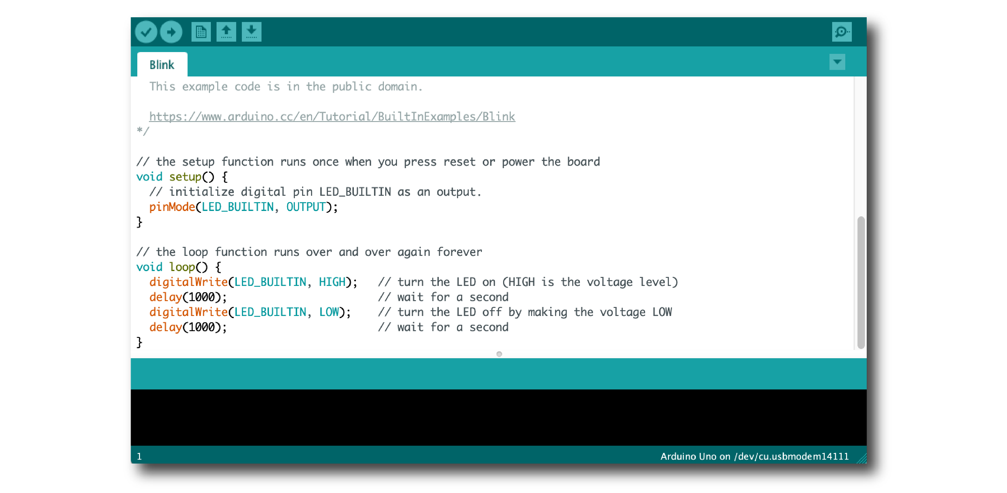
Connect the Arduino to the computer via USB
In the “Tools > Port” menu, make sure the correct device is selected
Use the “Upload” (right arrow) button to upload the Blink sketch to your device
When the sketch is successfully uploaded, a yellow LED on the Arduino should blink at 1 s intervals.
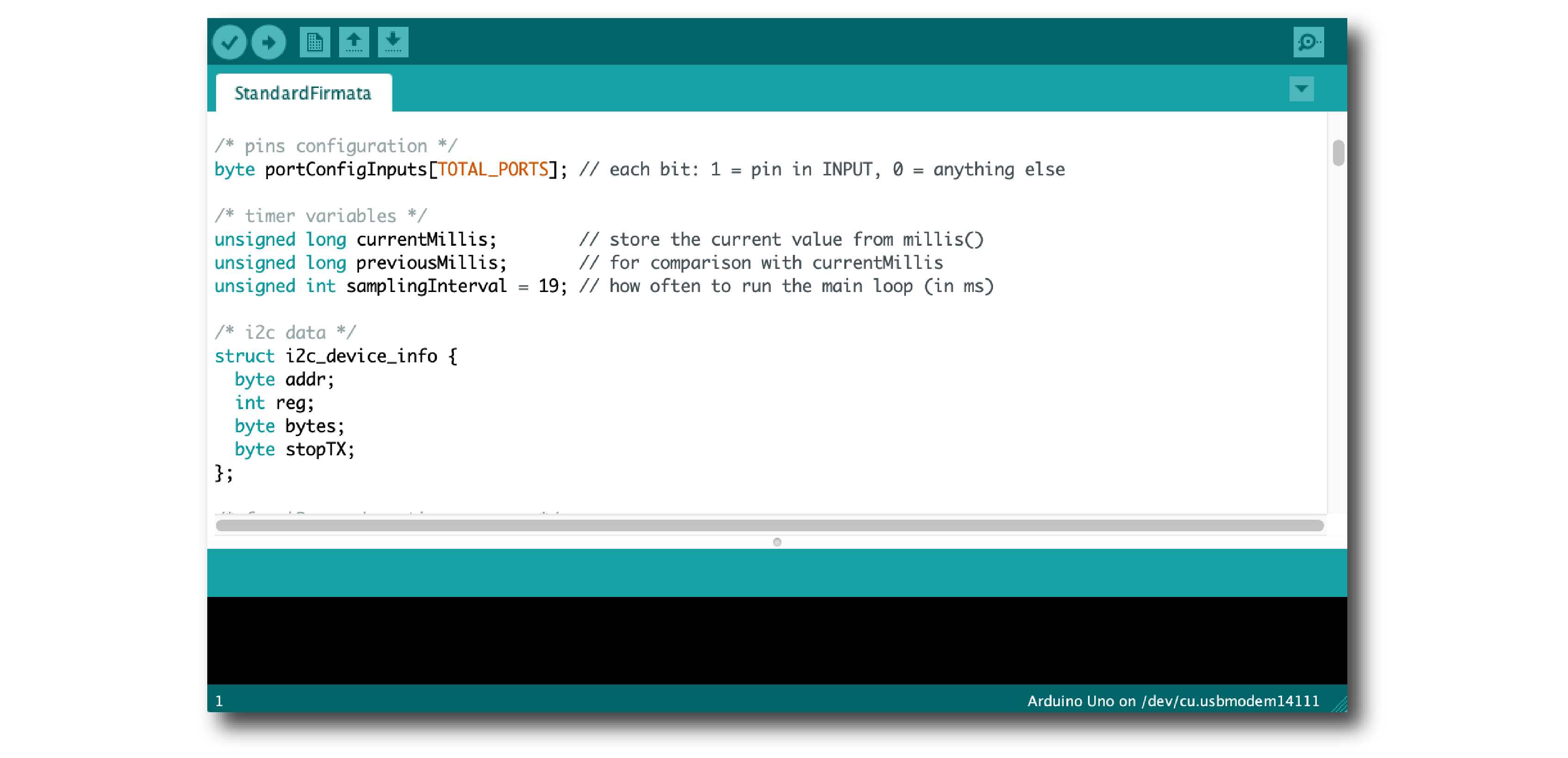
Arduino #2 will be delivering our feedback signal by communicating with the Arduino Output plugin inside the GUI. It can be substituted with another device that works with the GUI, such as a Pulse Pal from Sanworks.
To configure Arduino #2, follow the steps listed above, but upload the “File > Examples > Firmata > StandardFirmata” sketch:
Connecting the devices#
Once the Arduinos have been configured, connect the various devices according to the schematic below:
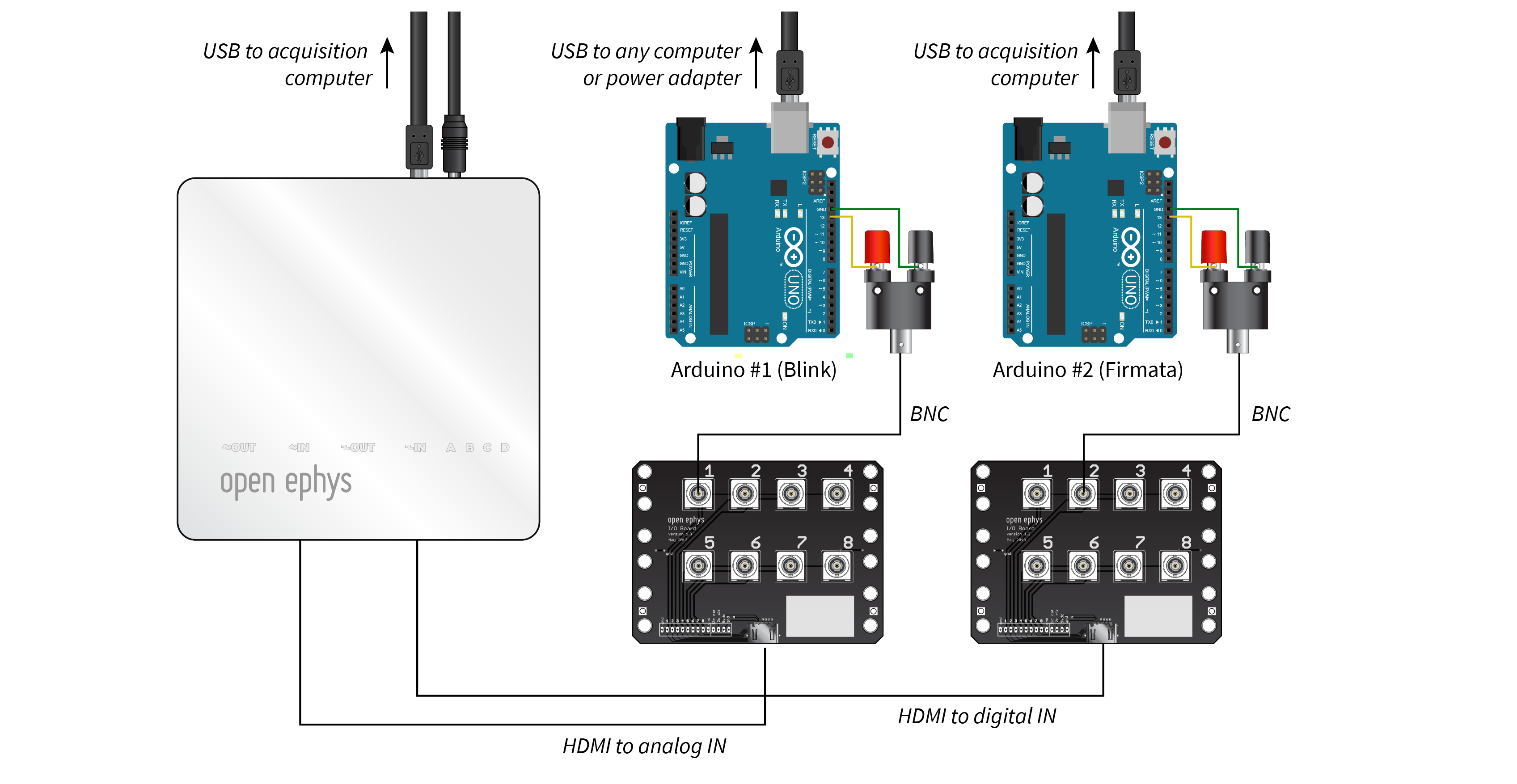
The acquisition board should be connected to the computer via USB.
I/O board #1 should be connected to the
ANALOG INPUTport (2nd from left) of the acquisition board via HDMI.I/O board #2 should be connected to the
DIGITAL INPUTport (4th from the left) of the acquisition board via HDMI.Arduino #1 should be powered via USB. Use the hookup wire to connect pin 13 to the positive (red) terminal of the BNC adapter and the ground pin to the negative (black) terminal of the BNC adapter.
Arduino #2 should be connected via USB to the same computer as the acquisition board. Use the hookup wire to connect pin 13 to the positive (red) terminal of the BNC adapter and the ground pin to the negative (black) terminal of the BNC adapter.
Use one BNC cable to connect the BNC adapter for Arduino #1 to input channel 1 of I/O board #1
Use the other BNC cable to connect the BNC adapter for Arduino #2 to input channel 2 of I/O board #2
Detecting incoming events#
Once all of the devices are connected, launch the Open Ephys GUI. Starting with an empty signal chain, add the following plugins, from left to right:
Acquisition Board - This plugin should automatically detect and connect to the Open Ephys acquisition board, assuming it’s connected to the computer. Press the “ADC” button to add the analog input channels to the data stream.
Crossing Detector - If this plugin does not appear in the signal chain, it can be added via the Plugin Installer (File > Plugin Installer). Press the “Constant” threshold button and change the value to 3. If there are headstages connected, set the input channel (upper left button) to the first ADC channel (number of headstage channels + 1). In the example below, there are 64 headstage channels, so the first ADC channel is 65.
LFP Viewer - Scroll down to channel ADC1 and double click on it so it fills up the whole display.
The signal chain should now look like this:
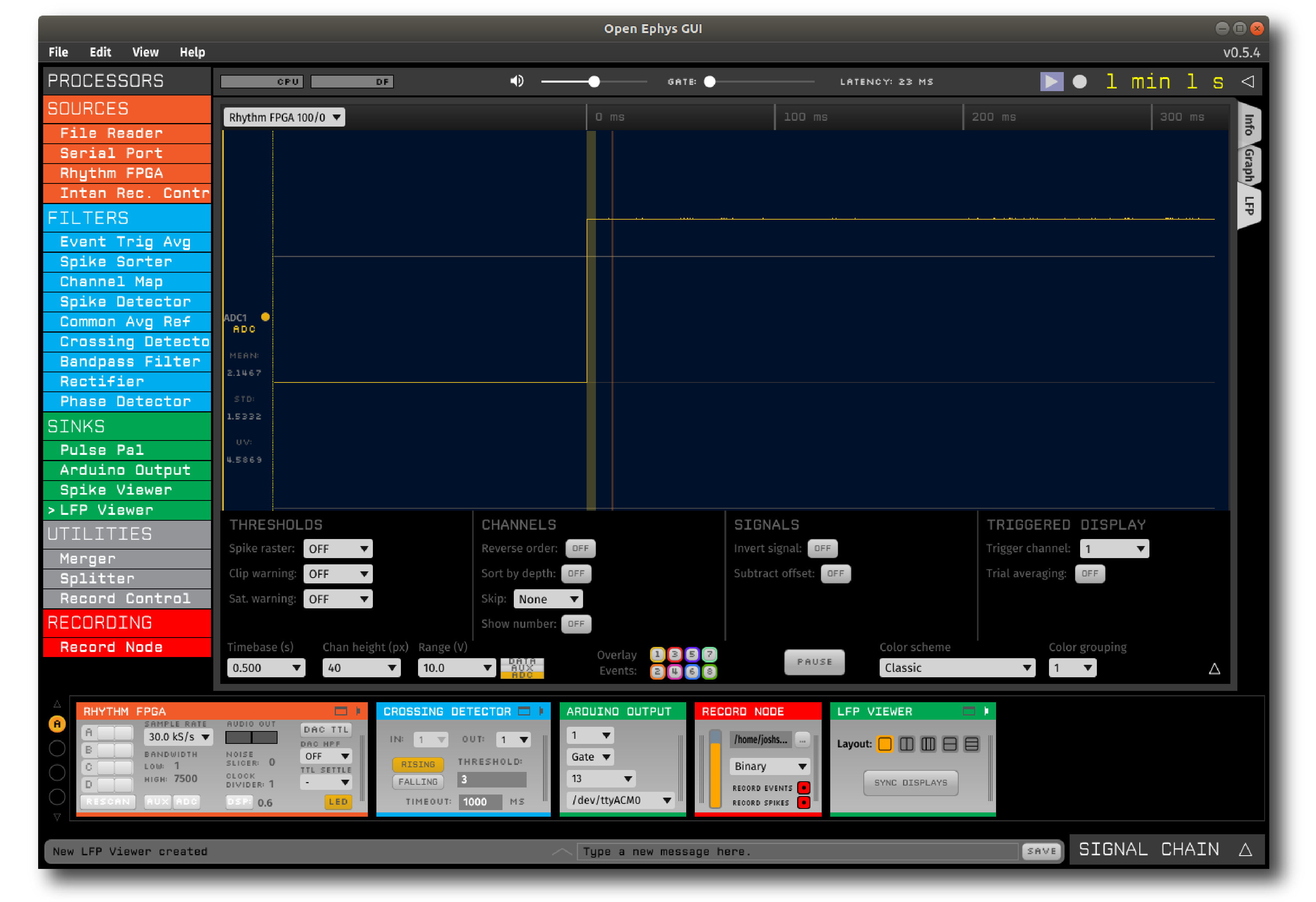
If you start acquisition, you should see digital events on TTL Line 1 (yellow translucent vertical bars) aligned with the onset of each pulse.
Tip
Setting the LFP Viewer to trigger when an event appears on channel 1 will ensure that the display is always aligned with the incoming events.
Generating digital outputs#
Next, we will add an Arduino Output plugin after the LFP Viewer, so our signal chain can create digital pulses in response to incoming events. Once the plugin has been added to the signal chain, make sure you’ve selected the Device that corresponds to Arduino #2, and the “Input line” is set to 1 (the same line used by the Crossing Detector).
If everything is connected correctly, you should now see two events associated with each pulse: one on line 1 (yellow) that’s perfectly aligned to the start, and one on line 2 (orange) that’s slightly offset in time. The pulse on line 2 is the one generated by Arduino #2:
Measuring system latency#
The final step is to measure the overall latency between the pulses on line 1 (when the input was received) and line 2 (when the response was generated). This can easily be done using the Latency Histogram plugin. If you don’t see this in your processor list, use the Plugin Installer to add it.
Drag and drop the Latency Histogram plugin after the Arduino Output. The default settings measure the latency between events on TTL Line 1 and TTL Line 2. Assuming the Crossing Detector is generating events on Line 1 and Arduino #2 is connected to Digital Input 2 of the acquisition board, these settings do not need to be adjusted.
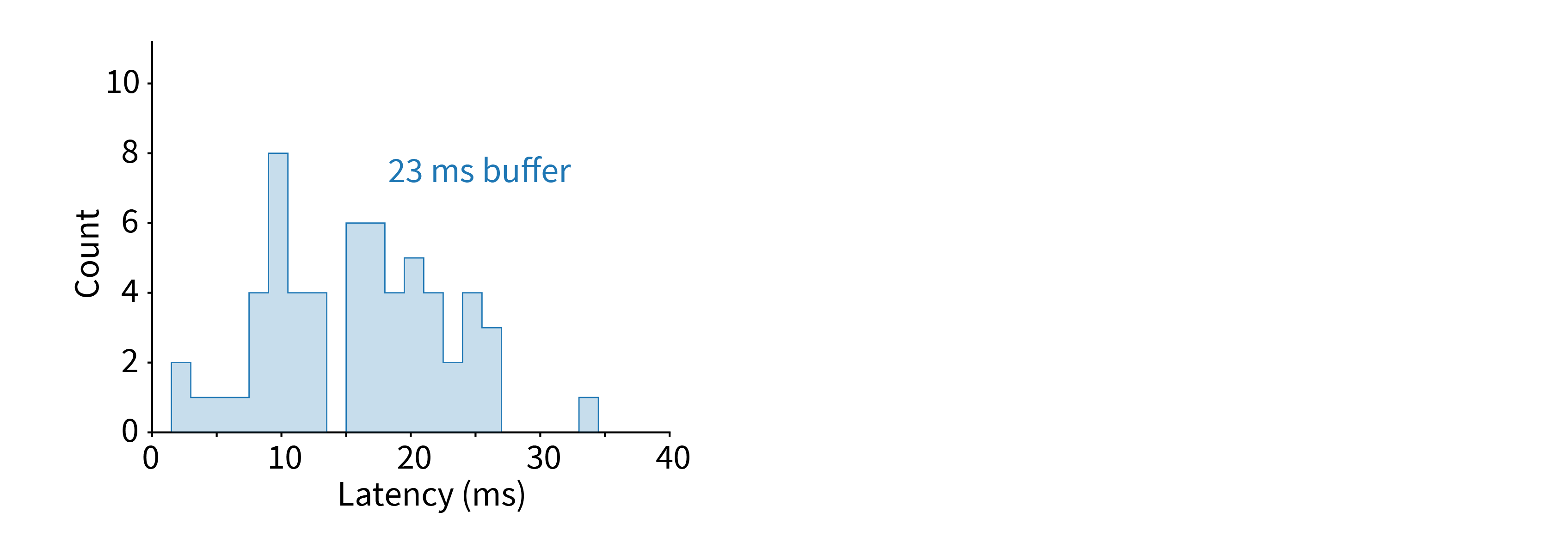
Start acquisition and let it run for a few minutes. The Latency Histogram plugin will build up a histogram of round-trip latencies, and also show the mean and standard deviation. In the example below, the latencies span between 0 and 27 ms, with a mean of 14 ms.
Settings that affect latency#
The Open Ephys GUI (and most other software for real-time processing) moves data around using buffers. Each buffer contains a block of samples for a set of channels. The larger the buffer (in terms of samples or channels), the more time it takes to process, and hence higher latency. However, larger buffers can typically have higher throughput, because the overhead involved in initiating each buffer exchange consumes a smaller fraction of overall processing time.
There are two types of buffers that affect the latency in this setup. The first is the hardware-to-software buffer that is used to transmit data between the acquisition board device and the Open Ephys GUI. Because the USB protocol has a high amount of overhead for each data packet, this buffer is set to 10 ms at 30 kHz. If using a different type of transmission interface (such as Ethernet or PCIe), much smaller buffer sizes are possible. Changing the size of this buffer for the Acquisition Board plugin requires editing the source code and re-compiling the GUI.
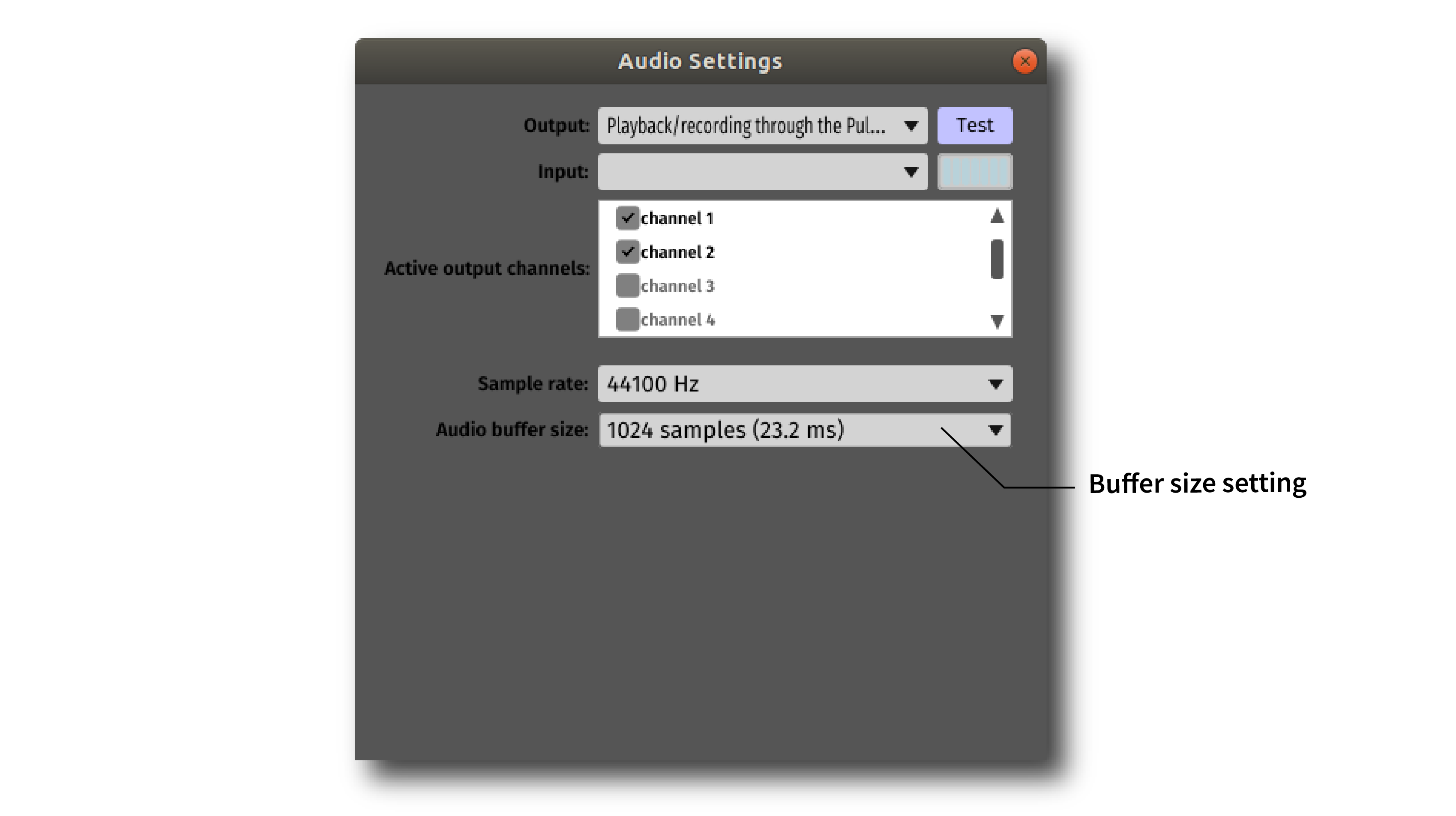
The second, and more easily configurable, type of buffer is the one used to pass data between plugins in the GUI’s signal chain. The size of this buffer can be changed by opening the “Audio Settings” interface, accessible via the “latency” button in the GUI’s control panel. The samples displayed in the latency interface are based on the sample rate of your computer’s audio card (44.1 kHz in most cases).
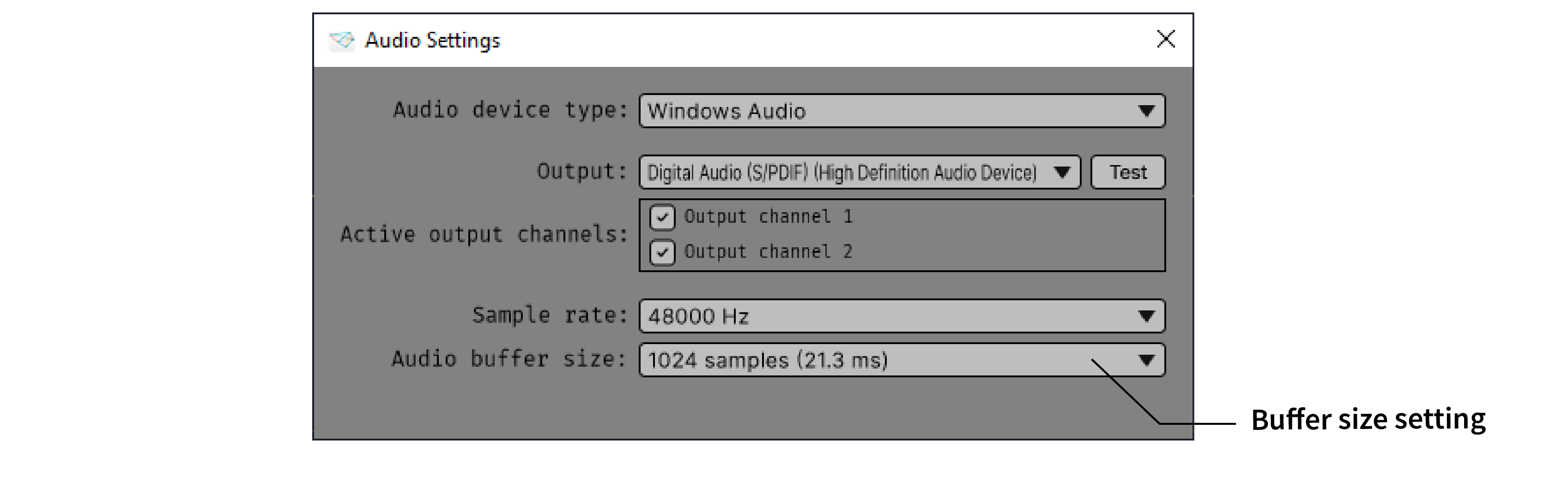
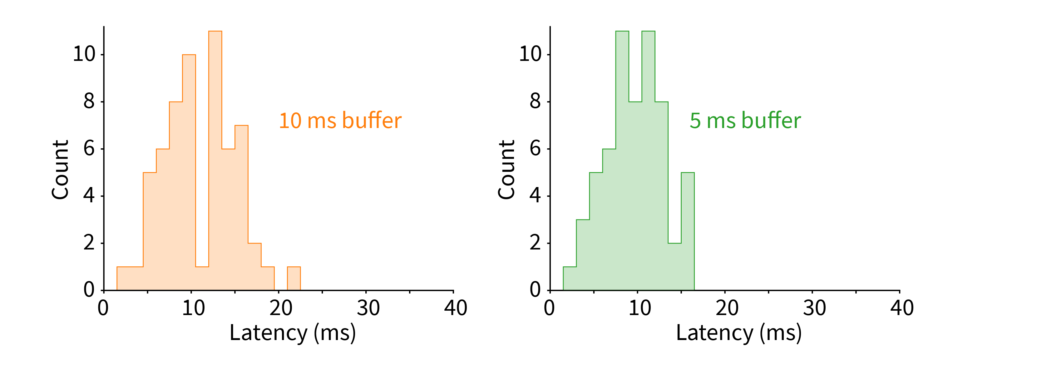
The default latency is around 20 ms, which works well for most open-loop signal chains. If you’re delivering closed-loop feedback, it may be desirable to use a lower latency setting. However, keep in mind that smaller buffers have lower throughput, which may cause the CPU meter to spike.
Here is what the same latency measurements look like for a 10 ms buffer size:
There may be diminishing returns for even smaller buffer sizes, due to the fact that overall latency is also limited by the size of the USB buffer on the acquisition board.
The minimum latency is also affected by the number of continuous channels that are being processed simultaneously. If your CPU meter is spiking for smaller buffer sizes, try reducing the number of continuous channels by disabling unused channels with a Channel Map plugin.
Next steps#
Once you’ve gotten the above setup working, it can be helpful to try using the File Reader plugin to trigger feedback. For example, you could a Bandpass Filter (between 4 and 12 Hz) in combination with the Phase Detector plugin to replicate the theta-phase-specific stimulation used in Siegle et al., 2014.