Binary Format#

Platforms |
Windows, Linux, macOS |
Built in? |
Yes |
Key Developers |
Aarón Cuevas López, Josh Siegle |
Source Code |
Advantages
Continuous data is stored in a compact format of tiled 16-bit integers, which can be memory mapped for efficient loading.
Additional files are stored as JSON or NumPy data format, which can be read using
numpy.loadin Python, or the npy-matlab package.The format has no limit on the number of channels that can be recorded simultaneously.
Continuous data files are immediately compatible with most spike sorting packages.
Limitations
Requires slightly more disk space because it stores one 64-bit sample number and one 64-bit timestamp for every sample.
Continuous files are not self-contained, i.e., you need to know the number of channels and the “bit-volts” multiplier in order to read them properly.
It is not robust to crashes, as the NumPy file headers need to be updated when recording is stopped.
File organization#
Within a Record Node directory, data for each experiment is contained in its own sub-directory. The experiment number is incremented whenever acquisition is stopped, which will reset the timestamps/sample numbers to zero. A new settings.xml file will be created for every experiment.
Experiment directories are further sub-divided for individual recordings. The recording number is incremented whenever recording is stopped, which will not reset the timestamps/sample numbers. Data from multiple recordings within the same experiment will have internally consistent timestamps/sample numbers, and will use the same settings.xml file.
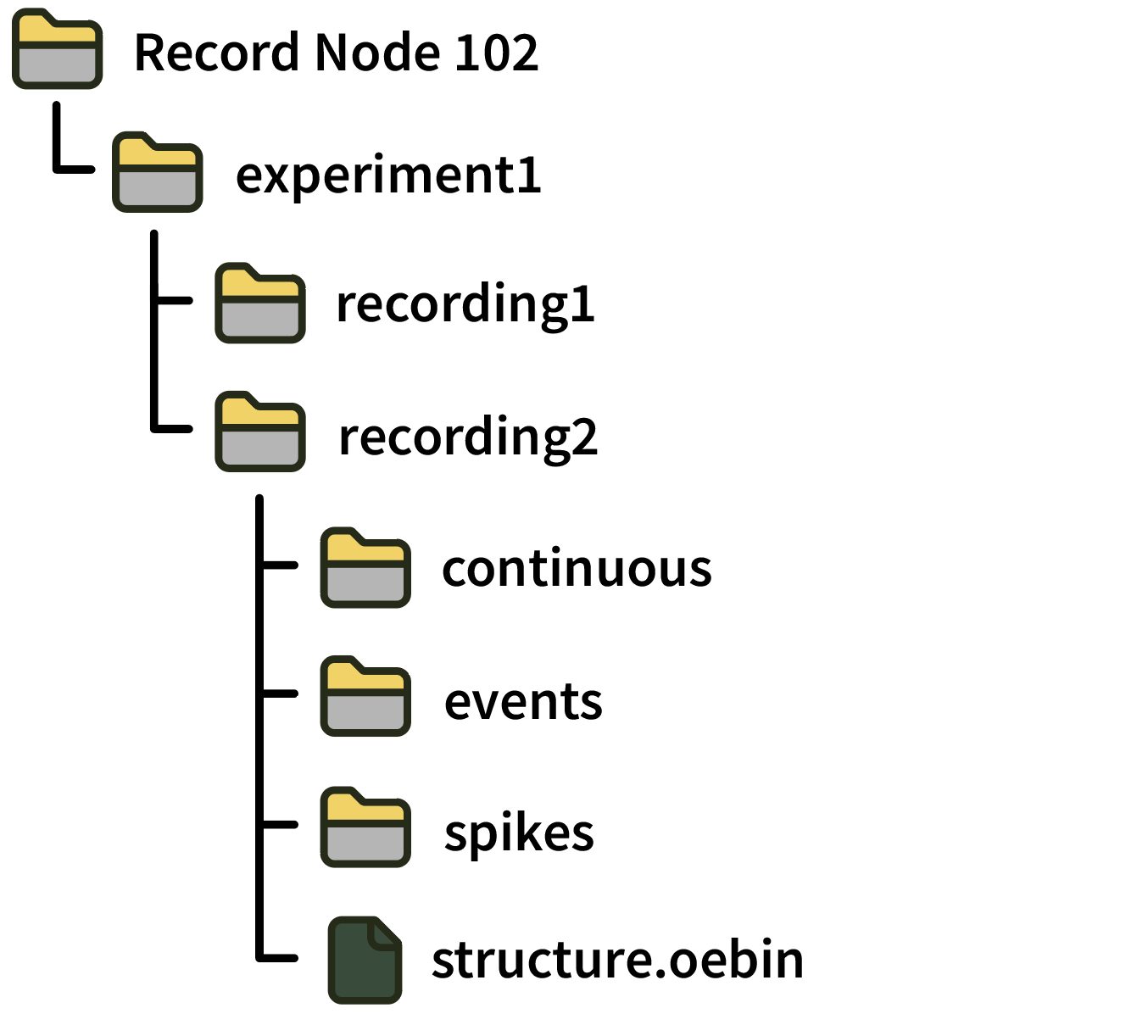
A recording directory contains sub-directories for continuous, events, and spikes data. It also contains a structure.oebin, which is a JSON file detailing channel information, channel metadata, and event metadata descriptions.
Format details#
Continuous#
Continuous data is written separately for each stream within a processor (a block of synchronously sampled channels):
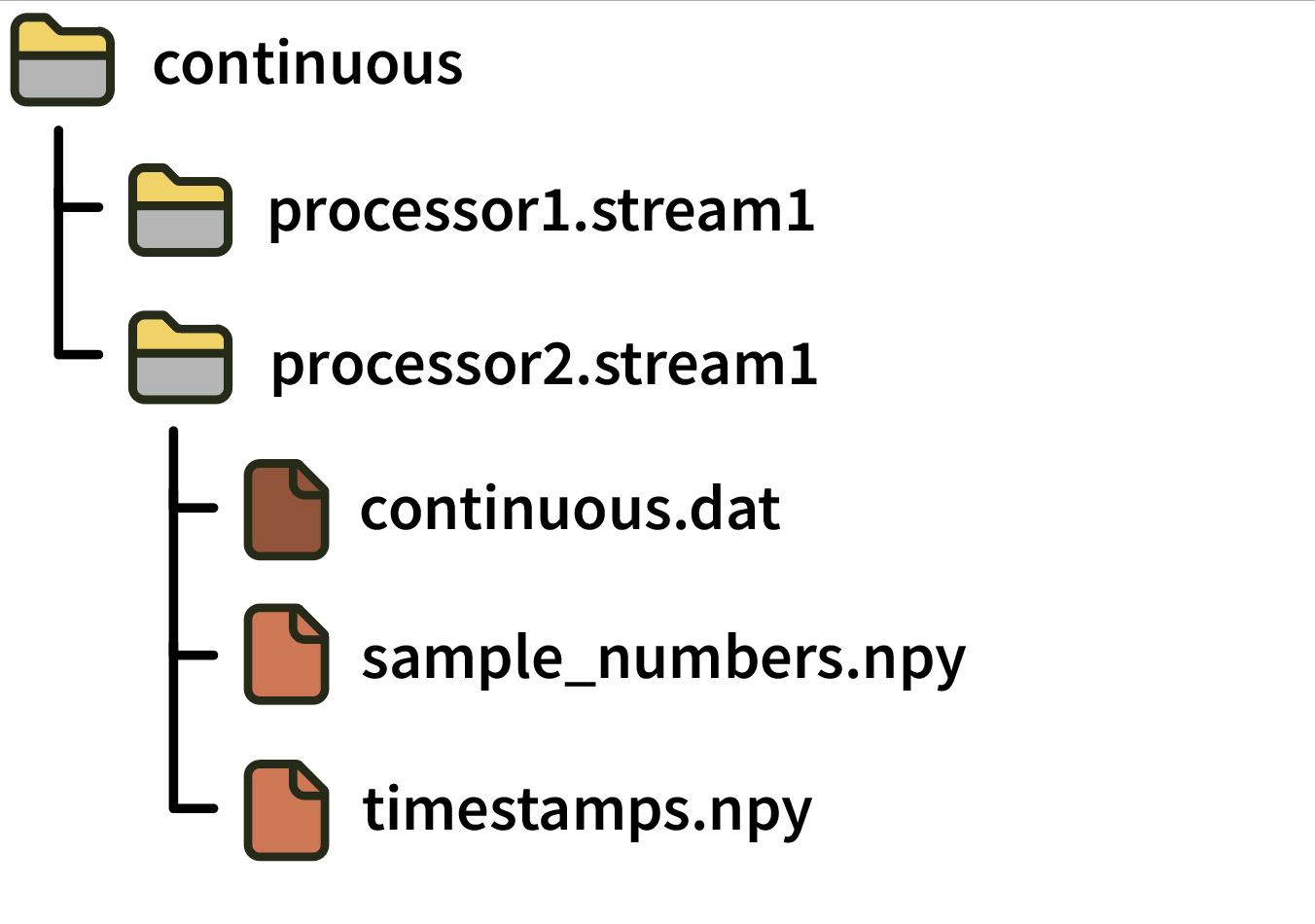
Each continuous directory contains the following files:
continuous.dat: A simple binary file containing N channels x M samples signed 16-bit integers in little-endian format. Data is saved asch1_samp1, ch2_samp1, ... chN_samp1, ch1_samp2, ch2_samp2, ..., chN_sampM. The value of the least significant bit needed to convert the signed 16-bit integers to physical units is specified in thebitVoltsfield of the relevant channel in thestructure.oebinJSON file. For “headstage” channels, multiplying bybitVoltsconverts the values to microvolts, whereas for “ADC” channels,bitVoltsconverts the values to volts.sample_numbers.npy: A numpy array containing M 64-bit integers that represent the index of each sample in the.datfile since the start of acquisition. Note: This file was calledtimestamps.npyin GUI version 0.5.X. To avoid ambiguity, “sample numbers” always refer to integer sample index values starting in version 0.6.0.timestamps.npy: A numpy array containing M 64-bit floats representing the global timestamps in seconds relative to the start of the Record Node’s main data stream (assuming this stream was synchronized before starting recording). Note: This file was calledsynchronized_timestamps.npyin GUI version 0.5.X. To avoid ambiguity, “timestamps” always refer to float values (in units of seconds) starting in version 0.6.0.
Events#
Event data is organized by stream and by “event channel” (typically TTL). Each event channel records the states of multiple TTL lines.
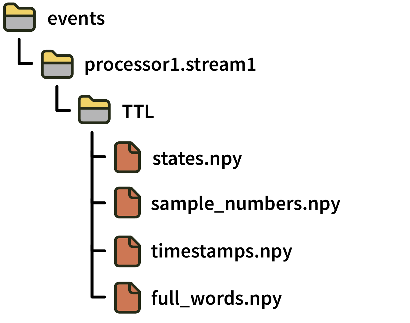
Directories for TTL event channels include the following files:
states.npy: numpy array of N 16-bit integers, indicating ON (+CH_number) and OFF (-CH_number) states Note: This file was calledchannel_states.npyin GUI version 0.5.X.sample_numbers.npyContains N 64-bit integers indicating the sample number of each event since the start of acquisition. Note: This file was calledtimestamps.npyin GUI version 0.5.X. To avoid ambiguity, “sample numbers” always refer to integer sample index values starting in version 0.6.0.timestamps.npyContains N 64-bit floats indicating representing the global timestamp of each event in seconds relative to the start of the Record Node’s main data stream (assuming this stream was synchronized before starting recording). Note: This file did not exist in GUI version 0.5.X. Synchronized (float) timestamps for events first became available in version 0.6.0.full_words.npy: Contains N 64-bit integers containing the “TTL word” consisting of the current state of all lines when the event occurred
Text events#
Text events are routed through the GUI’s Message Center, and are stored in a directory called MessageCenter. They contain the following files:
text.npy: numpy array of N stringssample_numbers.npyContains N 64-bit integers indicating the sample number of each text event on the Record Node’s main data stream. Note: This file was calledtimestamps.npyin GUI version 0.5.X. To avoid ambiguity, “sample numbers” always refer to integer sample index values starting in version 0.6.0.timestamps.npyContains N 64-bit floats indicating representing the global timestamp of each text event in seconds relative to the start of the Record Node’s main data stream. Note: This file did not exist in GUI version 0.5.X. Synchronized (float) timestamps for events first became available in version 0.6.0.
Spikes#
Spike data is organized first by stream and then by electrode.
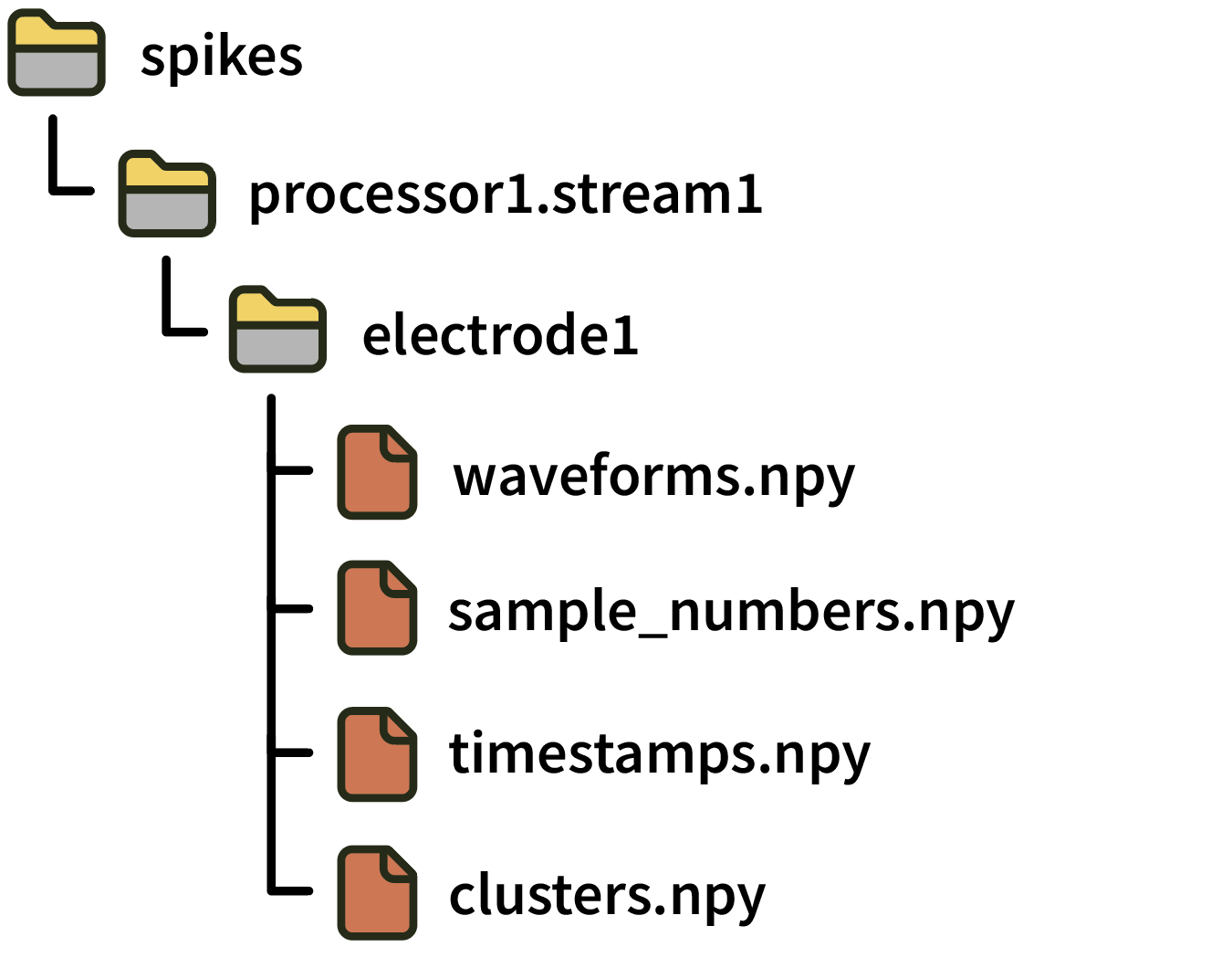
Each electrode directory contains the following files:
waveforms.npy: numpy array with dimensions S spikes x N channels x M samples containing the spike waveformssample_numbers.npy: numpy array of S 64-bit integers containing the sample number corresponding to the peak of each spike. Note: This file was calledtimestamps.npyin GUI version 0.5.X. To avoid ambiguity, “sample numbers” always refer to integer sample index values starting in version 0.6.0.timestamps.npy: numpy array of S 64-bit floats containing the global timestamp in seconds corresponding to the peak of each spike (assuming this stream was synchronized before starting recording). Note: This file did not exist in GUI version 0.5.X. Synchronized (float) timestamps for spikes first became available in version 0.6.0.clusters.npy: numpy array of S unsigned 16-bit integers containing the sorted cluster ID for each spike (defaults to 0 if this is not available).
More detailed information about each electrode is stored in the structure.oebin JSON file.
Reading data in Python#
Using open-ephys-python-tools#
The recommended method for loading data in Python is via the open-ephys-python-tools package, which can be installed via pip.
First, create a Session object that points to the top-level data directory:
from open_ephys.analysis import Session

session = Session(r'C:\Users\example_user\Open Ephys\2025-08-03_10-21-22')
The Session object provides access to data inside each Record Node. If you only had one Record Node in your signal chain, you can find its recordings as follows:
recordings = session.recordnodes[0]
recordings is a list of Recording objects, which is a flattened version of the original Record Node directory. For example, if you have three “experiments,” each with two “recordings,” there will be six total Recording objects in this list. The one at index 0 will be recording 1 from experiment 1, index 1 will be recording 2 from experiment 1, etc.
Each Recording object provides access to the continuous data, events, spikes, and metadata for the associated recording. To read the continuous data samples for the first data stream, you can use the following code:
samples = recordings[0].continuous[0].get_samples(start_sample_index=0, end_sample_index=10000)
print(f'Stream name: {recordings[0].continuous[0].metadata("stream_name")}')
This will automatically scale the data into microvolts before returning it.
To read the events for the same recording:
events = recordings[0].events
This will load the events for all data streams into a Pandas DataFrame with the following columns:
line- the TTL line on which this event occurredsample_number- the sample index at which this event occurredtimestamp- the global timestamp (in seconds) at which this event occurred (defaults to -1 if all streams were not synchronized)processor_id- the ID of the processor from which this event originatedstream_index- the index of the stream from which this event originatedstream_name- the name of the stream from which this event originatedstate- 1 or 0, to indicate whether this event is associated with a rising edge (1) or falling edge (0)
The fastest way to find the nearest continuous sample to a particular event is by using the np.searchsorted function:
import numpy as np
event_index = 100 # the index of the event you're interested in
event_timestamp = events.iloc[event_index].timestamp
nearest_continuous_sample_index = \
   np.searchsorted(recordings[0].continuous[0].timestamps,
                   event_timestamp)
For more information on how to use the open-ephys-python-tools library, check out this README
Using SpikeInterface#
You can also load data from the Open Ephys Binary format via SpikeInterface, using the read_openephys() method.
Reading data in Matlab#
Use the open-ephys-matlab-tools library, available via the Matlab File Exchange.