Open Ephys Format#

Platforms |
Windows, Linux, macOS |
Built in? |
Yes |
Key Developers |
Josh Siegle, Aarón Cuevas López |
Source Code |
Advantages
Data is stored in blocks with well-defined record markers, meaning data recovery is possible even if files are truncated by a crash.
The file header contains all the information required to load the file.
Limitations
Windows imposes a limit on the number files that can be written to simultaneously, meaning the Open Ephys format is not compatible with very high-channel-count recordings (>8000 channels).
In order to achieve robustness, files contain redundant information, meaning they use extra space and take longer to load.
File organization#
All data files are stored within the same Record Node directory, with a completely flat hierarchy. Files for different experiments have a number appended after an underscore (starting with _2 for the second experiment in a session). Data from different recordings is distinguished by the recording index values within each .spikes, continuous, or .events file.
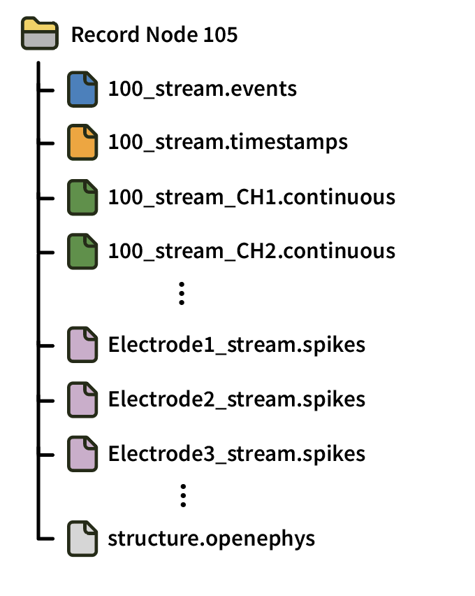
Each Record Node directory also contains at least one structure.openephys file, an XML file with metadata about the available files, as well as messages.events, a text file containing text events saved by the GUI.
Format details#
Headers#
All headers are 1024 bytes long, and are written as a MATLAB-compatible string with the following fields and values:
format = ‘Open Ephys Data Format’
version = 0.4
header_bytes = 1024
description = ‘(String describing the header)’
date_created = ‘dd-mm-yyyy hhmmss’
channel = ‘(String with channel name)’
channelType = ‘(String describing the channel type)’
sampleRate = (integer sampling rate)
blockLength = 1024
bufferSize = 1024
bitVolts = (floating point value of microvolts/bit for headstage channels, or volts/bit for ADC channels)
For those not using MATLAB, each header entry is on a separate line with the following format:
field names appear after a “header.” prefix
field names and values are separated by “ = “
the value of the field is in plain text, with intended strings enclosed in single quotes (as demonstrated above)
each line is terminated with a semicolon
Continuous#
Continuous data for each channel is stored in a separate .continuous file, identified by the processor ID (e.g. 100), stream name, and channel name (e.g. CH1). After the 1024-byte header, continuous data is organized into “records,” each containing 1024 samples.
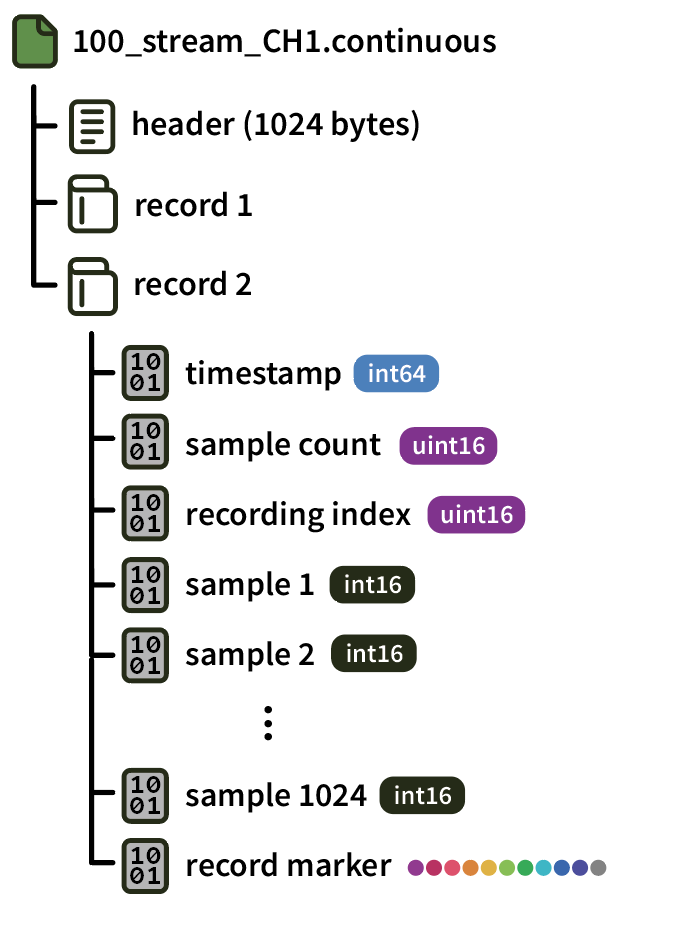
Each record is 2070 bytes long, and is terminated by a 10-byte record marker (0 1 2 3 4 5 6 7 8 255).
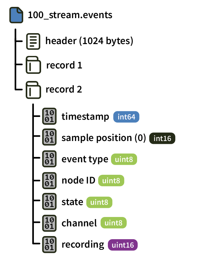
Events#
Events for each stream are stored in a .events file. Each “record” contains the data for an individual event stored according to the following scheme:
Spikes#
Data from each electrode is saved in a separate file. The filename is derived from the electrode name with spaces removed (e.g., “Electrode1”) and the data stream name.
Each record contains an individual spike event (saved for one or more channels), and is written in the following format:
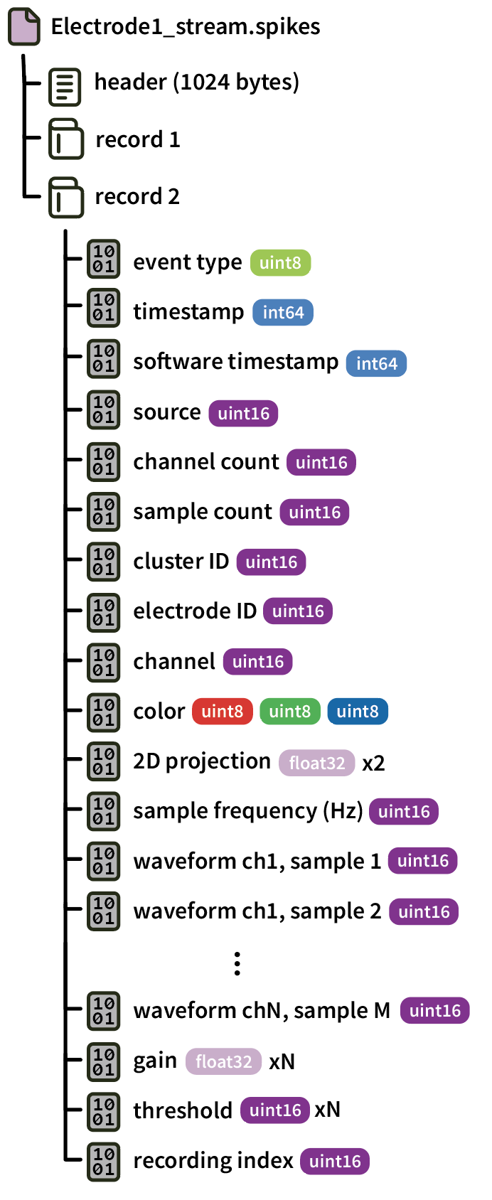
Since the samples are saved as 16-bit unsigned integers, converting them to microvolts involves subtracting 32768, dividing by the gain, and multiplying by 1000.
Reading data in Python#
Using open-ephys-python-tools#
The recommended method for loading data in Python is via the open-ephys-python-tools package, which can be installed via pip.
First, create a Session object that points to the top-level data directory:
from open_ephys.analysis import Session

session = Session(r'C:\Users\example_user\Open Ephys\2025-08-03_10-21-22')
The Session object provides access to data inside each Record Node. If you only had one Record Node in your signal chain, you can find its recordings as follows:
recordings = session.recordnodes[0]
recordings is a list of Recording objects, which is a flattened version of the original Record Node directory. For example, if you have three “experiments,” each with two “recordings,” there will be six total Recording objects in this list. The one at index 0 will be recording 1 from experiment 1, index 1 will be recording 2 from experiment 1, etc.
Each Recording object provides access to the continuous data, events, spikes, and metadata for the associated recording. To read the continuous data samples for the first data stream, you need to first set the sample range (to prevent all samples from being loaded into memory), and then call get_samples():
recordings[0].set_sample_range([10000, 50000])
samples = recordings[0].continuous[0].get_samples(start_sample_index=0, end_sample_index=10000)
print(f'Stream name: {recordings[0].continuous[0].metadata("stream_name")}')
This will automatically scale the data into microvolts before returning it.
To read the events for the same recording:
events = recordings[0].events
This will load the events for all data streams into a Pandas DataFrame with the following columns:
line- the TTL line on which this event occurredsample_number- the sample index at which this event occurredprocessor_id- the ID of the processor from which this event originatedstream_index- the index of the stream from which this event originatedstream_name- the name of the stream from which this event originatedstate- 1 or 0, to indicate whether this event is associated with a rising edge (1) or falling edge (0)
The fastest way to find the nearest continuous sample to a particular event is by using the np.searchsorted function:
import numpy as np
event_index = 100 # the index of the event you're interested in
event_timestamp = events.iloc[event_index].timestamp
nearest_continuous_sample_index = \
   np.searchsorted(recordings[0].continuous[0].sample_numbers,
                   event_sample_number)
For more information on how to use the open-ephys-python-tools library, check out this README
Using SpikeInterface#
You can also load data from the Open Ephys Binary format via SpikeInterface, using the read_openephys() method.
Reading data in Matlab#
Use the open-ephys-matlab-tools library, available via the Matlab File Exchange.